Testing probabilistic inference algorithms by estimating symmetrized KL divergences

Marco Cusumano-Towner - 01 Sep 2020

What does it mean for the inferences or judgments made by an artificially intelligent system (or for that matter, a human), to be correct? While this is a deep question with a large theoretical and applied literature that spans decades, the paradigm of probabilistic modeling and inference provides one coherent mathematical framework for addressing versions of this question. In turn, probabilistic programming systems, which reify the mathematical framework of probabilistic modeling and inference into reusable software infrastructure, can make it easier for users to test AI systems in light of a coherent definition of correctness.

There are a few key ideas in the probabilistic modeling and inference paradigm that support the development of coherent testing methodologies:

Key idea 1: Inferences take the form of probability distributions. An inference or prediction produced by a system takes the form of a probability distribution that encodes uncertain beliefs about some aspect of the past, present, or future state of the world.

Key idea 2: The prior assumptions can be encoded precisely: It is possible to precisely define the prior assumptions of the AI system in the form of a mathematical model, or better yet, a formal probabilistic modeling language within a probabilistic programming system. In this post, I will assume that the prior assumptions are represented as a probabilistic generative model, which has been encoded using a Gen modeling language.

Key idea 3: The correct distribution is well-defined. There are formulas from probability theory that compute the correct probability distribution that the system should produce, given its prior assumptions and the observed data and the quantity being inferred or predicted.

It is therefore possible in principle to test probabilistic AI systems by checking that their inferences or predictions match the correct probability distribution, or measuring how far they differ from the correct distribution. But there are at least two main challenges:

Challenge 1: Computing the correct distribution is often intractable. Except in highly specialized cases, or very small problems, it is usually not feasible to compute the correct probability distribution. Testing on special cases or small problems is necessary, but not sufficient, for building reliable AI systems.

Challenge 2: Comparing two distributions can be challenging: Even if we have computed the correct probability distribution, checking that the inferred distribution matches the correct distribution, or measuring the degree of difference between the distributions, is nontrivial. This task is made more complicated by the fact that there are various representations for probability distributions (e.g. a collection of samples, a black-box procedure that returns samples, a black-box probability mass or density function, a symbolic representation of the probability mass or density function, etc.). The techniques that can be used to compare distributions depend on how they are represented.

This post will mostly focus on the first challenge. We will restrict ourselves to testing inference procedures that produce distributions that support sampling and pointwise evaluation of their probability mass or density function. Specifically, I will introduce a methodology for testing probabilistic AI systems that is a special case of the AIDE technique introduced in our NeurIPS 2017 paper, and show how to implement it using the Gen probabilistic programming system. The techniques I will discuss in this post are based on a definition of correctness based on the Kullback-Leibler divergence between the inferred distribution and the correct distribution. I will show how the methodology can be used to evaluate the accuracy of (i) a variational inference procedure and (ii) a discriminative probabilistic model, for different observed data sets.

A generative model

The techniques I’ll describe are relevant to inference in any generative model, but I’ll use a model inspired by robotics as motivation. Suppose we are a robot moving around in a 2D plane, and we are trying to move to and pick up an object in the environment. Suppose we have a noisy object detector that returns a noisy measurement of the heading angle in the plane of the detection, relative to the heading of the robot, and suppose the robot has some prior beliefs about the location of the object. In order to rationally move through the environment towards the object, the robot needs to update its (unceratin) beliefs about the location of the object over time as it observes more detections.

Let’s start with a much simplified generative model of this scenario that includes a single time-step and no other objects in the environment, implemented in one of Gen’s modeling languages. The code below defines a generative model of the object’s location (x, y) and the noisy heading measurement measured_heading returned by the object detector. The robot is assumed to lie at the origin (0, 0) and to be facing down the positive x-axis (to the right from our birds-eye view).

using Gen

@gen function heading_model()
    x ~ normal(1.0, 1.0) # x-coordinate of object (a latent variable)
    y ~ normal(0.0, 1.0) # y-coordinate of object (a latent variable)
    heading = atan(y, x) # relative heading of the object (the robot is at the origin and facing down +x)
    measured_heading ~ von_mises(heading, 100.0) # measured relative heading
    return heading # for visualization and debugging purposes
end

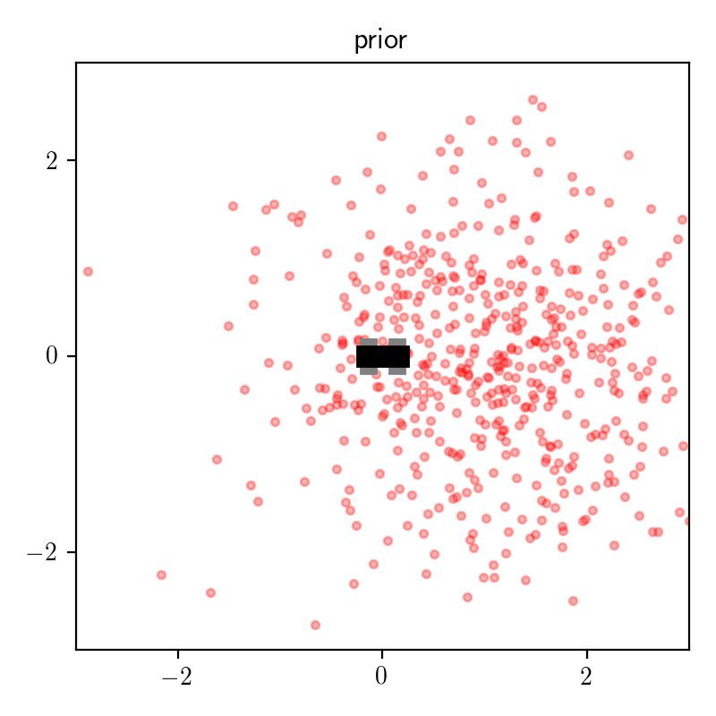
Let’s walk through this code briefly. The first two random choices, x and y, are the coordinates of the object. Here, the robot has a prior belief that the object is probably located somewhere in front of the robot (to the right in the birds-eye view). The plot below shows some samples of of (x, y) from the prior distribution:

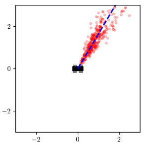
Next, theta = atan(y, x) computes the angle in radians of the object relative to the origin. Finally, we sample a random choice (obs) that represents the observed heading from a von Mises distribution centered at the true angle. The plots below show several joint samples from the prior, where the object location is a red dot, the true heading angle is shown as a solid blue line, and the observed heading angle is a dashed blue line:

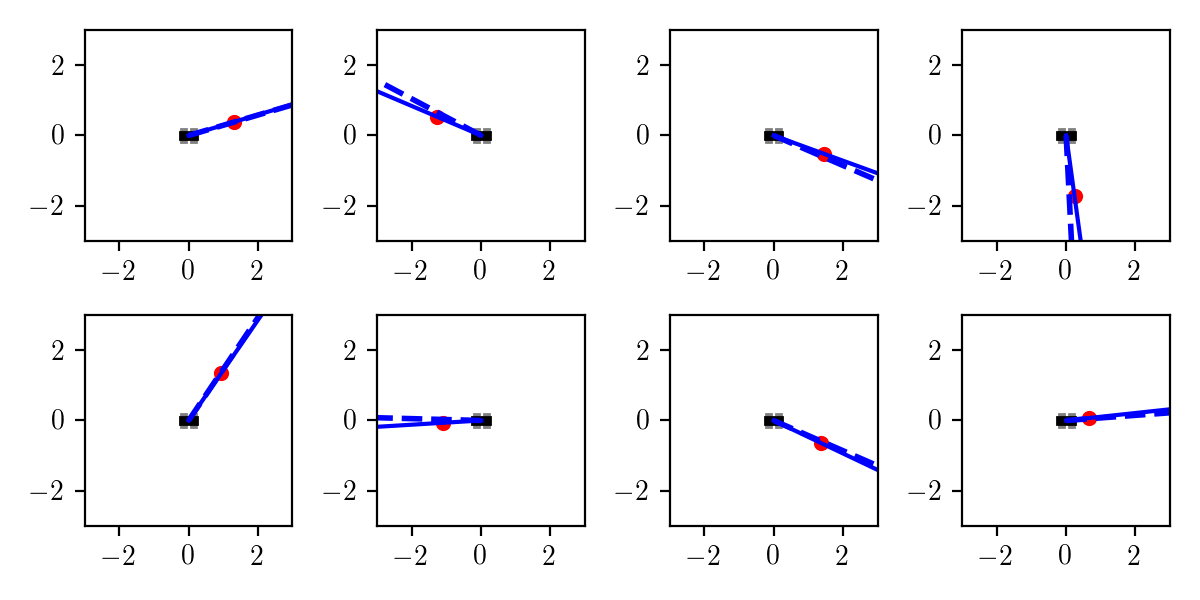
Each of these samples was generated using:

trace = Gen.simulate(heading_model, ())

Remember that a trace of a generative model in Gen includes both the latent and observed random choices. I wrote code for rendering a trace that can be used for visualizing the prior (as here) as well as inferences of different algorithms, as we will see shortly.

A simple Monte Carlo inference procedure

Given an observed relative heading measured_heading, we want to write an inference program that approximates the conditional distribution on x and y. Gen provides APIs for implementing a variety of customized Monte Carlo, variational, graph-based, and discriminative modeling approaches to inference (including hybrids), but because this is a low-dimensional problem, we can actually get a good approximation to the posterior distribution using a very basic importance sampling procedure:

(traces, log_normalized_weights, lml_estimate) = Gen.importance_sampling(
    heading_model, (), # the generative model and its argument (ours takes none)
    Gen.choicemap((:measured_heading, measured_heading)), # the observed data
    10000) # the number of importance samples

# resample 400 traces in proportion to weights, and extract x and y latents from them
weights = exp.(log_normalized_weights)
traces = [traces[Gen.categorical(weights)] for i in 1:400] 
xs = [trace[:x] for trace in traces]
ys = [trace[:y] for trace in traces]

Because I did not specify a custom proposal, this importance sampling procedure uses a default proposal based on forward sampling (also called ‘ancestral sampling’). Note that this is not intended to represent a typical Gen inference procedure— achieving efficient and accurate inferences in more complex problems typically requires more sophisticated inference code than this, and Gen’s primary purpose is to support development of much more sophisticated inference procedures. (Also note that in this post I am prefixing calls to the Gen library with Gen. to highlight them, even though this is technically unecessary since I already used using Gen.)

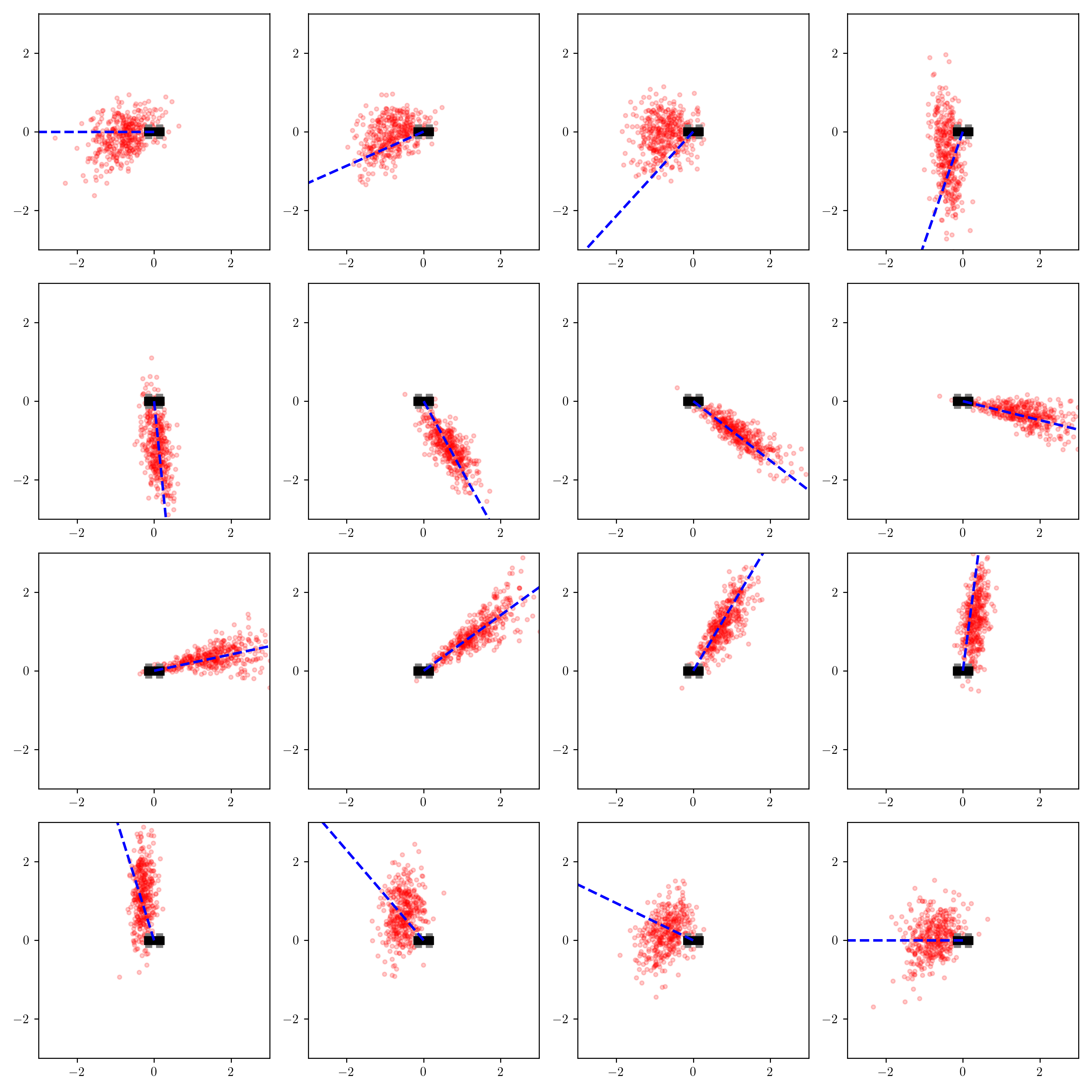
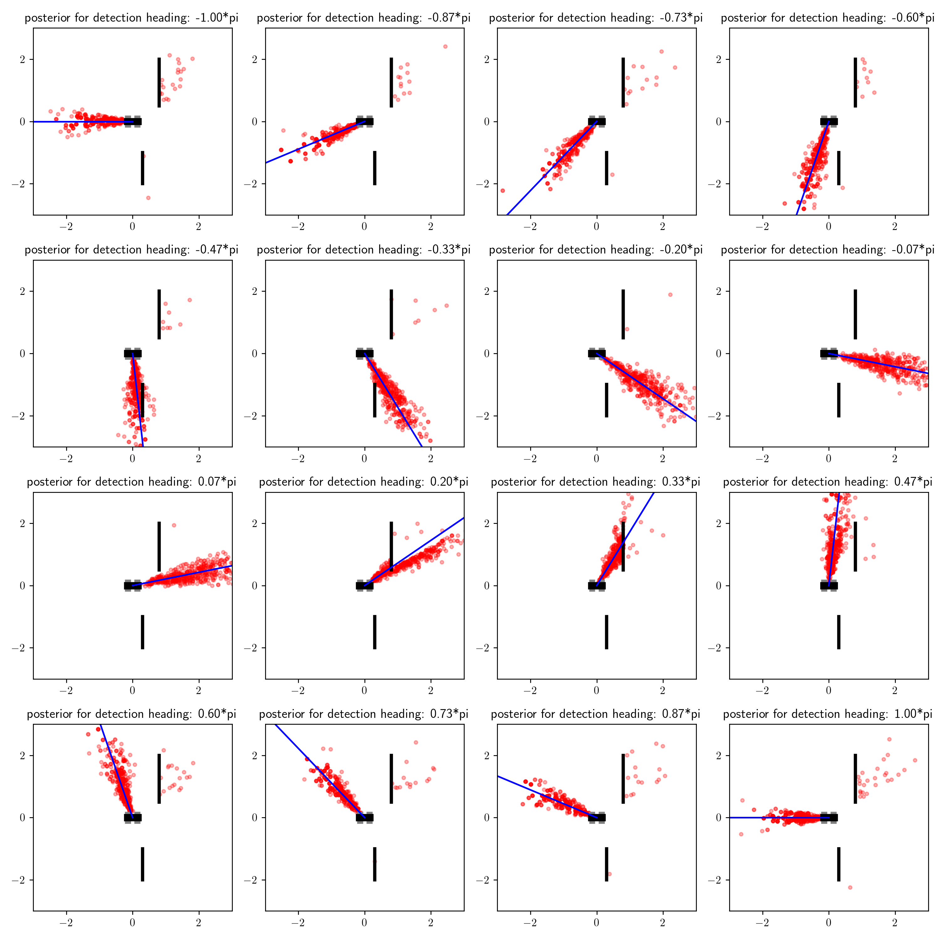
I ran the inference procedure above for 16 different values of measured_heading, and visualized the inferred conditional distribution on x and y for each one:

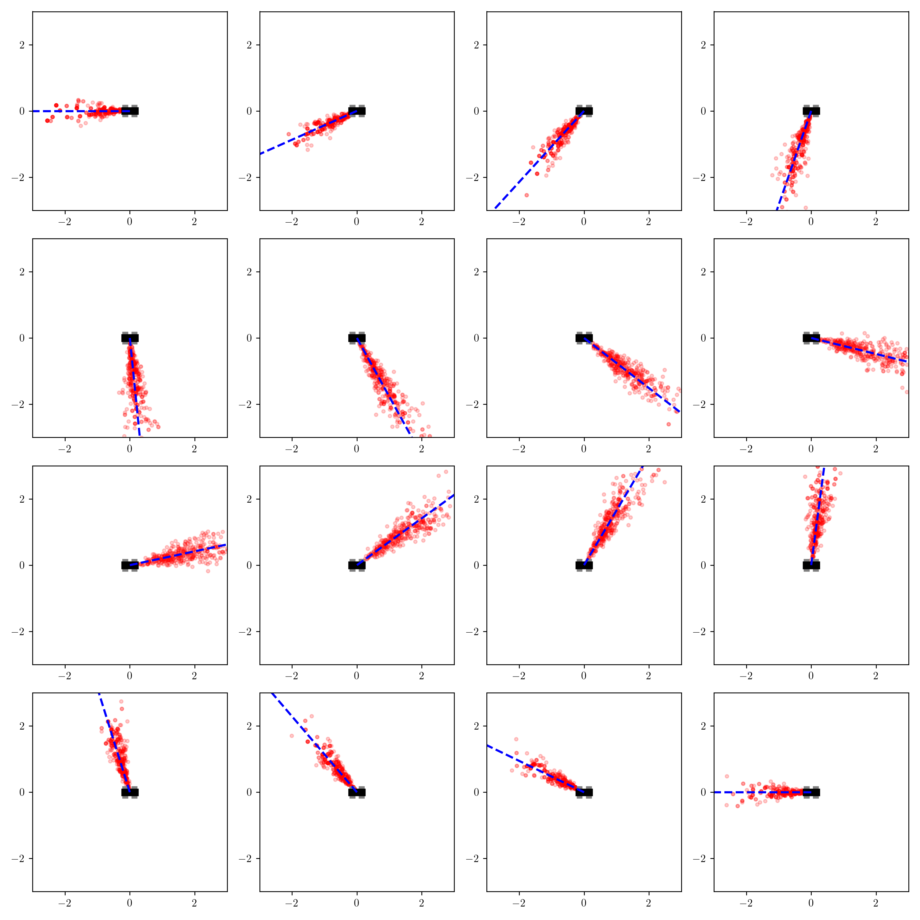
This result seems to make sense qualitatively. The robot believes the object is generally near the measured heading, with more uncertainty in the object’s exact position conditioned on the object being far away from the robot. One observation is that when the detection comes from behind the robot, the robot believes the object is probably closer to it than when the detection comes from in front of the robot.

One benefit of Monte Carlo algorithms is that they are often asymptotically exact, meaning that with enough computation, their output distribution converges to the correct distribution. This makes them useful for serving as ‘gold-standard’ distributions for testing more approximate but faster inference procedures, like variational inference and discriminative models. In later blog posts, I will describe techniques for testing Monte Carlo inference procedures themselves. This blog post will be focused on evaluating inference procedures whose results take the form of Gen generative functions. The key features of generative functions that we will use are (i) sampling from the distribution and (ii) evaluating its probability mass (or density) at given points in the latent space.

A simple variational inference procedure

One type of inference procedure that produces distributions represented as generative functions is variational inference. We will use Gen’s inference library implementation of black box variational inference, which is a class of algorithms introduced by Rajesh Ranganath et al. in a 2013 paper based on stochastic gradient descent that requires only the ability to evaluate the unnormalized log probability density of the model. Gen lets you apply black box variational inference using variational approximating families that are themselves defined as probabilistic programs (i.e. generative functions defined in one of Gen’s modeling languages).

The first step is to write a generative function that defines the variational approximating family. The generative function will have trainable parameters that we will optimize to match the true conditional distribution as closely as possible. To keep things simple, I’ll use a simple approximating family consisting of axis-aligned multivariate normal distributions:

@gen function q_axis_aligned_gaussian()
    @param x_mu::Float64
    @param y_mu::Float64
    @param x_log_std::Float64
    @param y_log_std::Float64
    x ~ normal(x_mu, exp(x_log_std))
    y ~ normal(y_mu, exp(y_log_std))
end

Then, we apply the procedure from Gen’s inference library to optimize the four parameters (x_mu, y_mu, x_log_std, and y_log_std):

# initialize parameters
Gen.init_param!(q, :x_mu, cos(measured_heading))
Gen.init_param!(q, :y_mu, sin(measured_heading))
Gen.init_param!(q, :x_log_std, 0.0)
Gen.init_param!(q, :y_log_std, 0.0)

# configure SGD update (initial step size 0.005, reduces to half after 100 iterations)
update = Gen.ParamUpdate(Gen.GradientDescent(0.005, 100), q_axis_aligned_gaussian)

# run black box variational inference, return final ELBO estimate
(elbo_est, _, _) = Gen.black_box_vi!(
    heading_model, (), # the generative model and its arguments (ours takes none)
    Gen.choicemap((:measured_heading, measured_heading)), # the observed data
    q_axis_aligned_gaussian, (), # the variational approximation and its arguments (ours takes none)
    update; iters=500, samples_per_iter=30) # optimization configuration

After optimizing the parameters for a particular value of measured_heading, we sample 400 times from the approximating distribution using Gen.simulate:

q_traces = [Gen.simulate(q_axis_aligned_gaussian, ()) for i in 1:400]

I ran the optimization routine separately for each value of measured_heading, and visualized the inferences using the same visualization code we used for the importance sampling inference procedure:

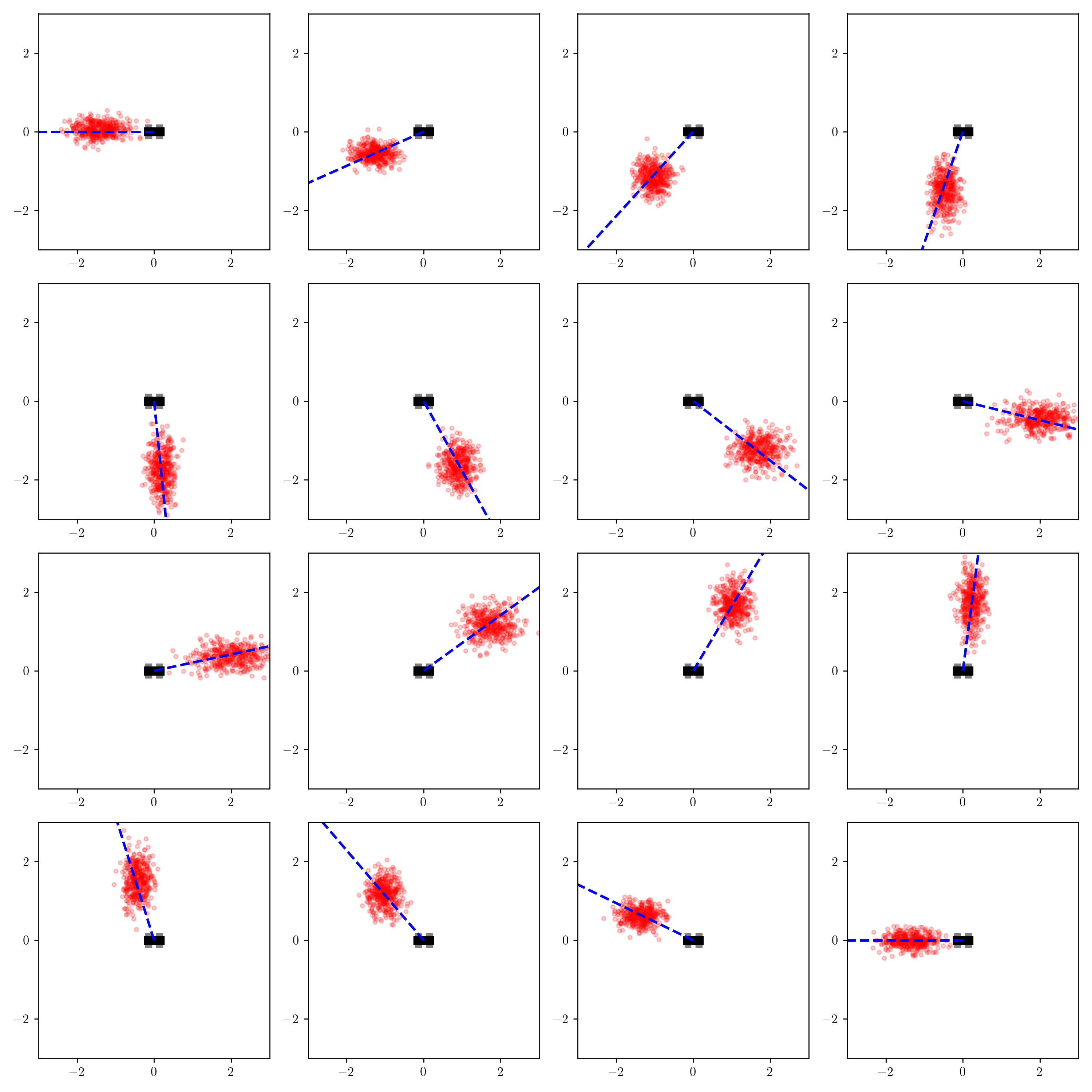
Compare these inferences to those from the importance sampling procedure. There are some clear qualitative differences. Consider the inferences for when measured_heading is near $\pi/4$:

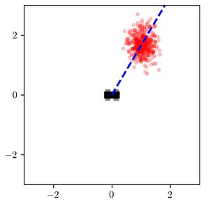
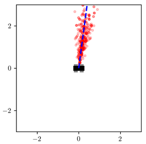
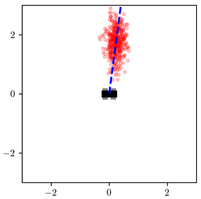
The variational distribution (right) places most of its probability mass near a certain distance away from the robot When measured_heading is $\pi/2$, the difference is less stark, but the variational distribution under-estimates the probability that the object is very close to the robot:

These results are not surprising. The variational family was too constrained to represent the shape of the posterior, and the objective function that it optimizes penalizes more heavily for placing probability mass in low-posterior-mass regions of the latent space than it does for assigning low-probability mass to high-posterior-mass regions (more on this shortly).

Instead of relying exclusively on manual qualitative comparisons like this for testing, we would like to automate the process of finding observations where the variational approximation is poor. We would also like to quantify the approximation error for different observed data sets, as opposed to just qualitatively compare the results. Finally, we would like general-purpose techniques that can be applied to various models.

One approach would be to discretize the latent space, and approximate each distribution by a discrete distribution on the discretized space by binning samples, and then compute a measure of the difference between the two discrete distributions, like a KL divergence. While that is conceptually relatively straightforward and useful in some situations, it is unsatisfactory as a general-purpose technique because the results will depend on the choice of discretization, and constructing the discretization can be difficult, especially in high-dimensional latent spaces. Another challenge is that we may not trust the Monte Carlo sampler to itself be accurate (more on this later!).

Using the evidence lower bound?

We will use the objective function of black box variational inference as the starting point for a quantitative evaluation of the approximation error. Let’s denote latent variables by $z$, observed variables by $x$, variational parameters by $\theta$, the density function for the variational approximating family by $q(\cdot; \theta)$ and the generative model joint density by $p(z, x)$.

Briefly, black box variational inference attempts to maximize the ‘evidence lower bound’ or ‘ELBO’:

Recall that maximizing the ELBO is equivalent to minimizing the ‘exclusive’ KL divergence:

Instead of comparing against a ‘gold-standard’ Monte Carlo sampler, we could try to employ this KL divergence as a measure of error to use to evaluate variational inference procedures. However, while is straightforward to estimate the ELBO by sampling from the variational approximation, it is not straightforward to estimate this KL divergence itself because the actual log marginal likelihood $\log p(x)$ is unknown, .

To illustrate the issue, I fit the variational family q_axis_aligned_gaussian for each of 200 evenly spaced values of measured_heading. The ELBO estimates at the end of the optimization for each value of measured_heading are shown below:

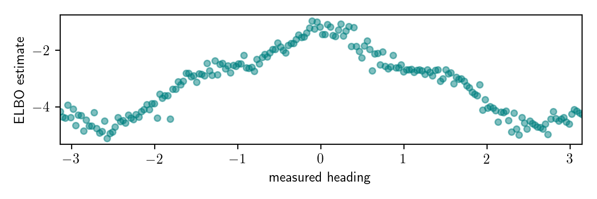
While this plot looks interesting, it does’t really give us much information about how accurate our variational inference procedure is for different observed data. While it looks like the ELBO is higher for measured_heading near 0, we don’t know how much to attribute this to higher marginal likelihood for these observations versus lower KL divergence.

For any given observed value of measured_heading, we don’t know the gap between the ELBO and the actual log marginal likelihood, so we can’t tell from this plot when our algorithm has high error. Also, the plot doesn’t tell us how the accuracy of the variational approximation depends on the observation.

Estimating the log marginal likelihood using Monte Carlo?

Fortunately, Monte Carlo algorithms can be used to accurately estimate the log marginal likelihood $\log p(x)$. We can use a Monte Carlo algorithm to estimate the log marginal likelihood for different data sets (i.e. different values of measured_heading), and then we can estimate the (exclusive) KL divergence as the difference between the log marginal likelihood estimate and the ELBO. Conveniently, the importance sampling procedures in Gen’s inference library return a log marginal likelihood estimate in addition to the collection of weighted samples (lml_estimate):

(traces, log_normalized_weights, lml_estimate) = Gen.importance_sampling(
    heading_model, (), # the generative model and its argument (ours takes none)
    Gen.choicemap((:measured_heading, measured_heading)), # the observed data
    10000) # the number of importance samples

This procedure is sufficient for accurately estimating the log marginal likelihood in this problem, but in general more sophisticated Monte Carlo techniques are needed. Gen’s inference libraries can also be used to implement annealed importance sampling (AIS), which is a gold-standard log marginal likelihood estimation technique, in a few lines of code. Various sequential Monte Carlo and MCMC techniques can also be used (indeed AIS is intimately related to both).

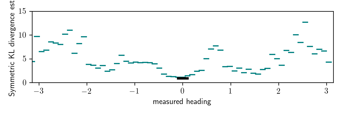
Below I plotted the log marginal likelihood estimates from importance sampling (IS) in yellow, on the left alongside the ELBO estimates from black box variational inference (BBVI). On the right, I show the KL divergence estimate obtained by taking the difference.

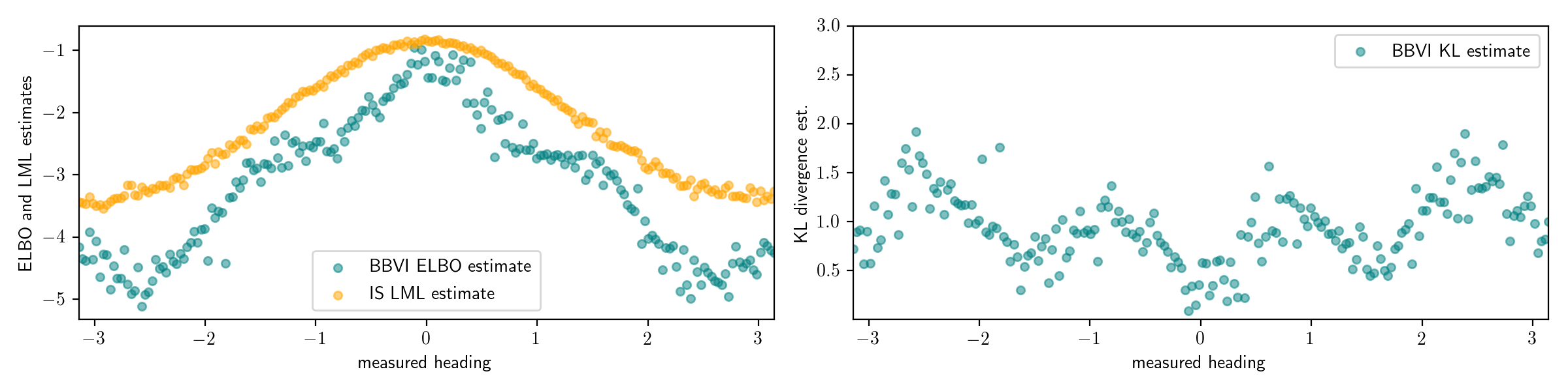
The KL divergence estimates on the right show an interesting pattern. The KL divergence is low for values of measured_heading near $-\pi/2$, $0$, $\pi/2$, $\pi$, (and $-\pi$), and high for values near $-\pi/4$, $\pi/4$, $-3\pi/4$, and $3\pi/4$. The procedure has correctly identified the issue we found by hand earlier, where the variational family is not able to capture the form of the posterior distribution for observed data in these regimes near $-\pi/4$, $\pi/4$, $-3\pi/4$, and $3\pi/4$. Additionally, the procedure is also able to quantify the error in the inferences. We now have a general-purpose technique for quantifying the error of variational inference procedures, based on a gold-standard Monte Carlo algorithm that estimates the log marginal likelihood. While this technique does require developing a gold-standard Monte Carlo algorithm for the problem, it importantly does not require ad-hoc model-specific choices like discretization of the latent space.

However, a potential weakness of this procedure is that it depends on the accuracy of the gold-standard Monte Carlo algorithm. Suppose we had run the importance sampling procedure with only 100 importance samples, instead of the 10,000 that were used above. Then, this importance sampling procedure significantly under-estimates the marginal likelihood, and the KL divergence estimates are in turn under-estimated; in some cases they are even negative (recall that the KL divergence is always non-negative):

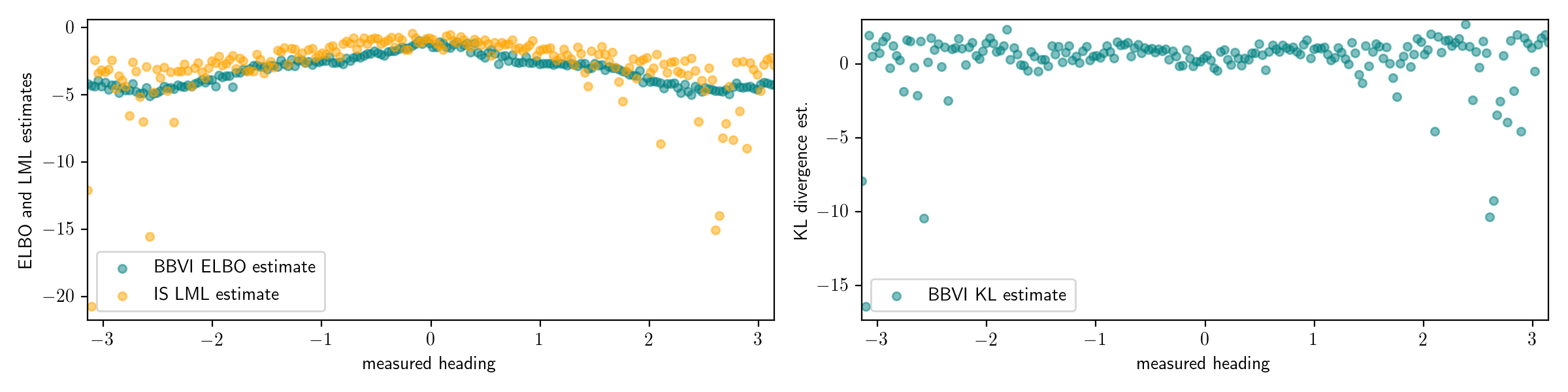
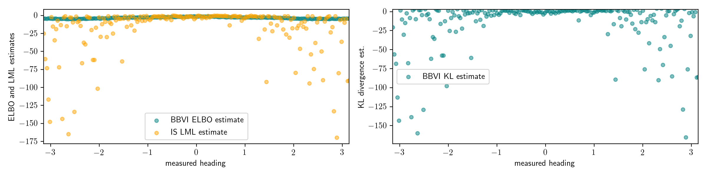
If we had estimated the log marginal likelihood with only 10 particles, the results would be even worse:

This problem is a deep one. Recall that the log marginal likelihood involves an integral over the entire latent space:

This is intrinsically hard in the worst case for any estimation procedure that is limited to evaluating $p(z, x)$ and without prior knowledge about properties of $p$, because $p(z, x)$ could be very large in very small and difficult-to-find parts of the latent space. (see Chapter 29 of David MacKay’s book for a beautiful analogy explaining the difficulty of posterior inference and integration).

Another weakness with the approach described in this section is that even if we could estimate the log marginal likelihood accurately, the exclusive KL divergence is not an ideal general-purpose measure of inference error: It can be small even when the variational approximation completely fails to capture modes of the correct conditional distribution. See here for an illustration and here for an interactive tool for exploring KL divergences.

Estimating symmetrized KL divergences for simulated data

It turns out that we could address both of the issues above (reliance on difficult-to-trust estimation of the log marginal likelihood and use of the exclusive KL divergence) if we had access to a sampler for the exact conditional distribution $p(\cdot | x)$. Consider the symmetrized KL divergence:

The symmetrized divergence is a better measure of accuracy than the exclusive divergence alone for many applications because it significantly penalizes the variational approximation for missing modes of the true conditional distribution. It turns out that if we have access to exact conditional samples, we can sidestep the estimation of the marginal likelihood and directly estimate the symmetrized KL divergence:

This is a difference between two terms. The first is an upper bound on the log marginal likelihood, and the second is the standard ELBO. We can estimate the ELBO as usual for variational inference. If we have access to an exact conditional sampler, then we can estimate the first term by sampling from the exact conditional distribution and evaluating $\log p(z, x) - \log q(z; \theta)$, and averaging the results.

You might be wondering how we could possibly expect to obtain exact conditional samples. Suppose that instead of an estimate of the symmetrized KL divergence for a specific $x$, we were instead willing to accept an estimate of the expected symmetrized KL divergence, over $x$ sampled from the prior $p(\cdot)$:

Note that here I have made the dependence of the variational parameters on $x$ in the notation explicit using $\theta(x)$. Also note that if the optimization process itself is stochastic (which it often is), then we could add an inner expectation over this randomness as well without significantly changing the interpretation. I will elide this randomness for the time being. The expected symmetrized KL divergence is then:

Note while sampling $z$ from $p(\cdot | x)$ for some given $x$ may be difficult, we can sample $z$ and $x$ jointly from $p$ easily, by calling Gen.simulate on the generative model. It is straightforward to construct a Monte Carlo estimator for the expected symmetrized KL divergence:

The code below samples $z_i$, $x_i$, and $z_i’$ and computes the quantity inside the sum of the estimator using Gen’s primitives. Note that this code is easily generalized to work for any generative model and any variational approximation. Also note that the simplicity of the code leverages the fact that generative models and variational approximations are represented in the same way, as generative functions which support a set of basic operations like Gen.simulate and Gen.generate and Gen.get_score. These are just a few of the operations in Gen’s generative function interface.

# simulate 'ground truth' latents and observed data jointly from the model
model_trace = Gen.simulate(heading_model, ())

# evaluate joint probability density of model for simulated latents and observed data
model_forward_score = Gen.get_score(model_trace)

# extract just the observed data
observation_choices = Gen.get_selected(Gen.get_choices(model_trace), Gen.select(:measured_heading))

# fit the variational approximation to the observed data
.. (see code above)

# evaluate probability density of variational approximation on the 'ground truth' latents
(_, approximation_backward_score) = Gen.generate(
    q_axis_aligned_gaussian, (), Gen.get_choices(model_trace))

# simulate latents from the variational approximation
approximation_trace = Gen.simulate(q_axis_aligned_gaussian, ())

# evaluate joint probability density of variational approximation
approximation_forward_score = Gen.get_score(approximation_trace)

# evaluate joint probability density of model on the latents from the variational approximation
(_, model_backward_score) = Gen.generate(
    heading_model, (),
    merge(observation_choices, Gen.get_choices(approximation_trace)))

# combine to form unbiased estimate of symmetric KL divergence for the synthetic observed data
symmetric_kl_estimate = (
    get_score(model_trace) - approximation_backward_score +
    get_score(approximation_trace) - model_backward_score)

The plot below shows the results of running the code above 1000 times. Each x-coordinate a simulated value of the observed data (measured_heading), and the y-coordinate is the corresponding value of symmetric_kl_estimate.

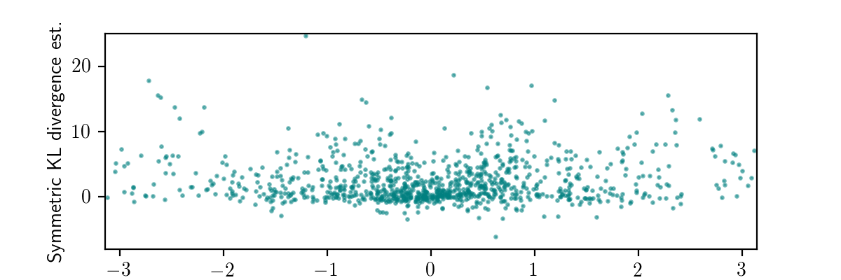
We could average all of the symmetric_kl_estimate values, and obtain an unbiased estimate of the average case symmetrized KL divergence for our black box variational inference procedure. In this case, we would get a value around 2.4525.

This testing procedure satisfies many of our objectives:

• It is general-purpose, and can be used with any generative model and variational inference procedure (provided the KL divergences are finite—more on this later!).

• It does not require heuristic choices like (i) test functions, (ii) discretizations of the latent space.

• It does not require trust in any ‘gold-standard’ inference procedure.

• It applies equally to discrete and continuous latent spaces, and does not require a metric on the latent space.

• It penalizes inference procedure being evaluated for missing modes of the posterior.

But we paid a heavy cost for these benefits: The procedure estimates an average-case error, where the expectation is taken under the distribution on observed data $x$ of the model. We can’t use the procedure to investigate the error of an inference procedure on a specific data set, or how error varies across data sets. The estimates also give low weight to data sets that are considered unlikely or rare under the model. However, the evaluation may still be useful in some settings for detecting bugs in inference procedures, or for optimizing the amount of computation used, or for comparing different inference procedures on the same objective footing,

A small modification to the procedure allows us to overcome this weakness to some degree. Instead of sampling $z$ and $x$ jointly from $p(\cdot)$, we can choose any event $E$ in the sampling space of observed data, and sample from $z$ and $x$ jointly from $p(\cdot | x \in E)$ via rejection sampling. Specifically, to estimate the average-case symmetrized KL divergence for observed data sets in $E$, we simply simulate traces from the generative model repeatedly and only accept those traces for which $x \in E$.

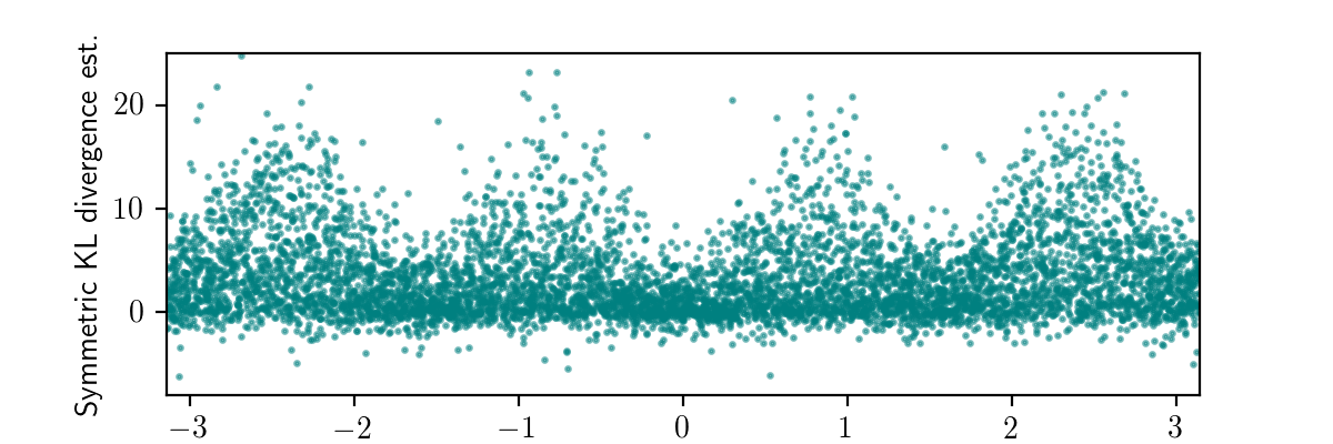
I applied this modification to the working example, by selecting $E$ to be an interval of width $\pi/32$ in which measured_heading must lie. In particular, I discretized the entire space of observations into 64 bins of this form, and applied rejection sampling until I got 100 traces within each bin, for a total of 6400 traces. Then, for each of these traces, I ran the code above to obtain a value of symmetric_kl_estimate. The plot below shows the results for all 6400 traces.

Next, we can average the values within each bin to obtain an unbiased estimate of the expected symmetrized KL divergence between the exact conditional distribution and the inference procedure’s variational distribution for data sets within the bin:

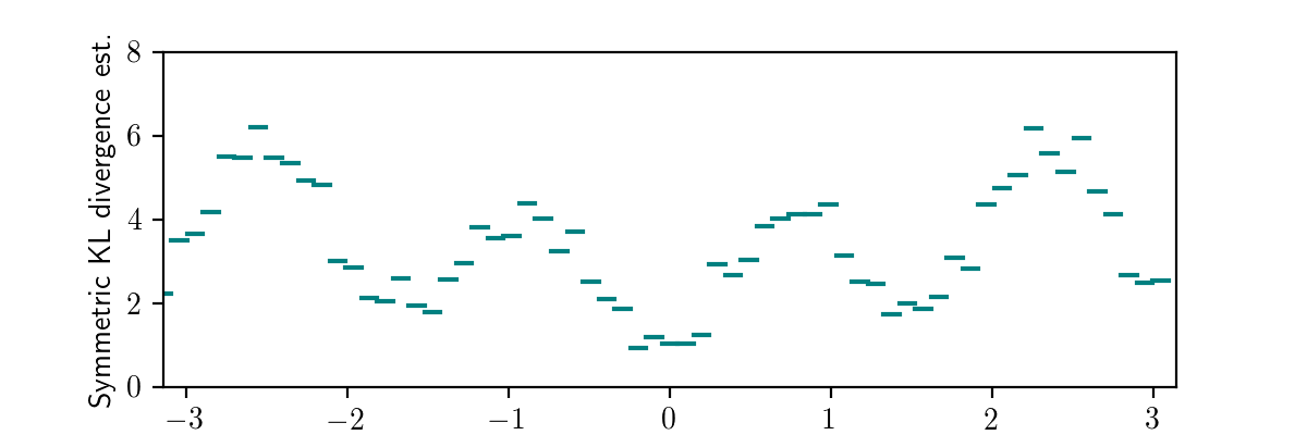
This plot again aligns with our earlier qualitative investigation as well as the automated quantitative testing based on a Monte Carlo log marginal likelihood estimation, but (i) does not assume accurate marginal likelihood estimation and (ii) significantly penalizes missing modes because it uses the sum of the ‘inclusive’ and ‘exclusive’ KL divergences. Progress!

Testing a discriminative inference network

We can use the procedure above to test any inference procedure that produces a generative function as its output. This includes variational inference, as well as discriminative probabilistic models based on neural networks. Next I’ll show how to define an inference network in Gen, how to train it data simulated from the generative model, and I’ll use the testing procedure we just derived above to compare the inference network and our black box variational inference procedure.

Below is a generative function called q_amortized that represents an inference network. Like the generative function q_axis_aligned_gaussian, this generative function samples two random choices x and y. However, it takes observed data (heading) an argument, and passes the heading through a neural network that computes the parameters of the distributions of x and y. This generative function also is able to represent dependence between x and y in its distribution, unlike q_axis_aligned_gaussian.

@gen function q_amortized(heading)
    @param b1::Vector{Float64}
    @param W1::Matrix{Float64}
    @param b2::Vector{Float64}
    @param W2::Matrix{Float64}
    @param b3::Vector{Float64}
    @param W3::Matrix{Float64}
    hidden1 = sigmoid.(b1 .+ (W1 * [heading, cos(heading), sin(heading)]))
    hidden2 = sigmoid.(b2 .+ (W2 * hidden1))
    output = b3 .+ (W3 * hidden2)
    x ~ normal(output[1], exp(output[2]))
    y ~ normal(output[3] + (output[4] * x), exp(output[5] + (output[6] * x)))
end

This of generative function, which accepts observed data as its argument and samples values for latent variables, could be trained like a discriminative model on real data as in straightforwrad supervised learning, or on data generated from a generative model (as in the sleep-phase of the wake-sleep algorithm), or by maximizing the expected ELBO as in a variational autoencoders. Some of these possibilities are discussed in the Gen documentation under Learning Generative Functions.

The code below trains the generative function q_amortized on data simulated from the generative model heading_model. Note that this corresponds to the following optimization problem:

where $\phi$ represents the parameters b1, W1, b2, and so on. That is, we are minimizing the expected ‘inclusive’ KL divergence, where the expectation is taken under the distribution of observed data expected by the generative model.

using Flux.Optimise
using GenFluxOptimizers: FluxOptimConf
num_hidden1 = 20
num_hidden2 = 20
num_output = 6
Gen.init_param!(q_amortized, :b1, zeros(num_hidden1))
Gen.init_param!(q_amortized, :W1, randn(num_hidden1, 3) * 0.1)
Gen.init_param!(q_amortized, :b2, zeros(num_hidden2))
Gen.init_param!(q_amortized, :W2, randn(num_hidden2, num_hidden1) * 0.1)
Gen.init_param!(q_amortized, :b3, zeros(num_output))
Gen.init_param!(q_amortized, :W3, randn(num_output, num_hidden2) * 0.1)
update = Gen.ParamUpdate(FluxOptimConf(Optimise.ADAM, (0.1, (0.9, 0.999))),
    q_amortized => [:b1, :W1, :b2, :W2, :b3, :W3])

# generate training data
ntrain = 100000
training_data = []
for i in 1:ntrain
    trace = simulate(heading_model, ())
    push!(training_data, (((trace[:measured_heading],), Gen.get_choices(trace))))
end

# train the parameters of q_amortized
objectives = Float64[]
minibatch_size = 100
for iter in 1:1000

    # obtain a minibatch
    permuted = Random.randperm(ntrain)
    minibatch = permuted[1:minibatch_size]
    
    # compute gradient for this minibatch
    total_log_weight = 0.0
    for (inputs, constraints) in training_data
        (trace, log_weight) = Gen.generate(q_amortized, inputs, constraints)
        total_log_weight += log_weight
        Gen.accumulate_param_gradients!(trace)
    end
    push!(objectives , total_log_weight / minibatch_size)
    
    # apply the SGD update and reset the gradients
    Gen.apply!(update)
end

After running the training code, I visualize the output distributions of q_amortized for the same grid of measured_heaing values that I used to visualize the output distributions of the importance sampler and the variational approximation q_axis_aligned:

The results are interesting. The inferences appear somewhat more accurate than those from black box variational inference when measured_heading is between $-\pi/2$ and $\pi/2$ (when the measurement comes from the front-side of the robot), but much less accurate when the measurement comes from the left-side of the robot. But we should also keep in mind that the inferences are much faster than those from black box variational inference because we only need to run the (quite small) neural network, as opposed to running an optimization algorithm.

Let’s see if our automated testing procedure is able to detect the high error of our trained inference network when the measurement comes from behind the robot. Below are the raw symmetric_kl_estimate values for a large number of randomly sampled measured_heading values.

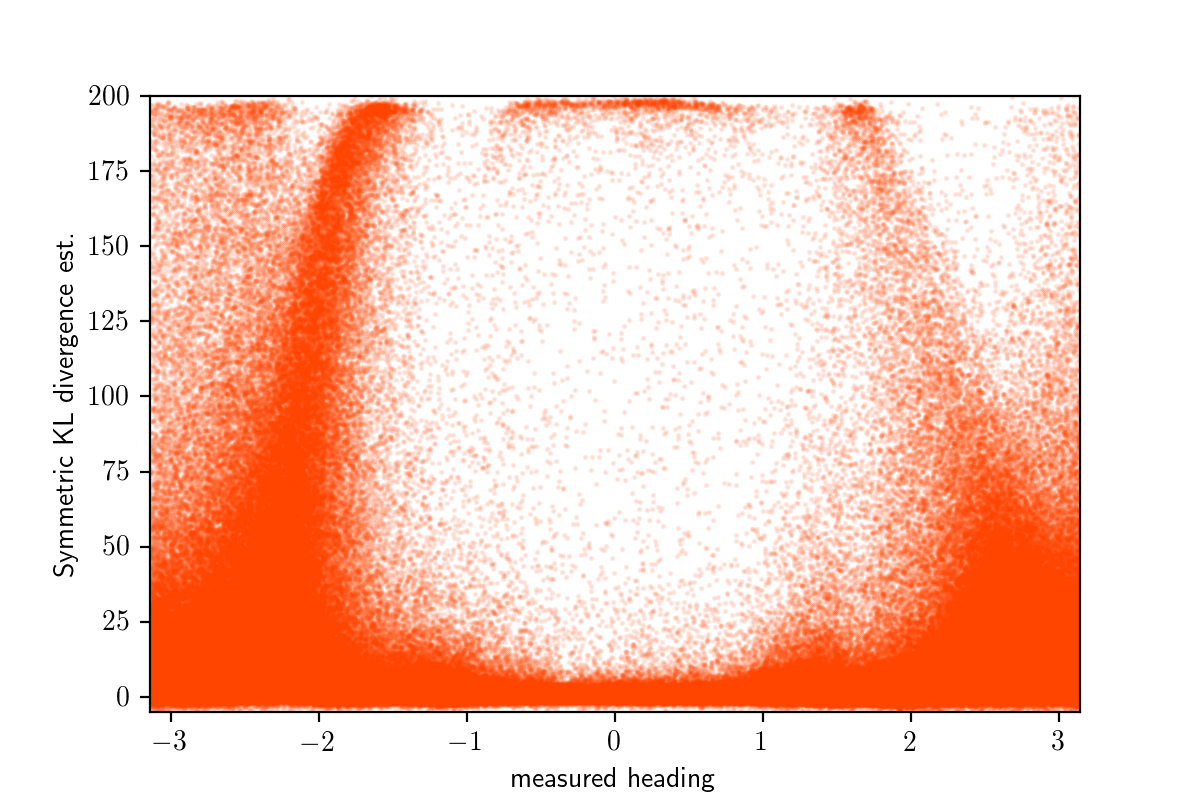
Averaging over bins as before, we get the per-bin symmetrized KL divergence estimates shown in orange below:

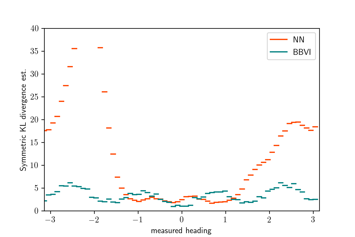
This plot confirms what we saw by a manual inspection. The error of q_amortized after training is similar or better than that of variational inference when measured_heading is in $[-\pi/2,\pi/2]$ and much worse outside this range. After reflecting on the objective function on which q_amortized was trained, this should not be surprising: Because the model’s prior distribution places most mass on scenarios where the object is in front of the robot, relatively few training examples have the measurement coming from behind the robot. Because the training procedure minimizes the average-case error, the network is willing to sacrifice accuracy on these relatively uncommon data sets if this allows it to be a little more accurate on the data sets that it believes are more common. This is an instance of a more general challenge with achieving robust inferences from to maximize discriminative models trained to maximize the expected log likelihood of the data.

Aside: Estimating error on specific observed data sets

If the set of the observed data $E$ on which we want to test average error is small enough (i.e. have very low probability $p(x \in E)$), then eventually generating traces for which $x \in E$ will become the bottleneck for the testing procedure outlined above. To illustrate this, I animated the rejection sampling process that I used to generate 100 traces within each of the 64 bins of measured_heading:

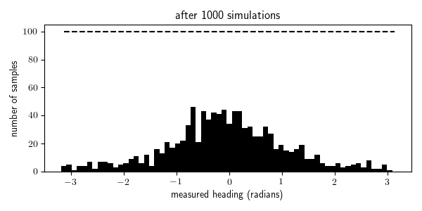
We see that we were able to generate all the traces needed for the bins with high prior probability (where the measurement comes from in front of the robot, in the range $[\pi/4, \pi/4]$) after a few thousand iterations, but it takes 10 times longer to generate all the traces needed for the bins with the lowest prior probability (where the measurement comes from behind the robot, near $\pi$ and $-\pi$). Indeed it takes, in expectation, $N/p(x \in E)$ simulations from the generative model to obtain $N$ samples for which $x \in E$ where $p(x \in E)$ is the probability that $x \in E$ according to the generative model. In problems with higher-dimensional observation spaces, we need to take care not to define the events $E$ to be too specific.

In the limiting case where we want to test error on a particular observed data set, the procedure above will not suffice. But it turns out the procedure can be modified to work on particular data sets, if we are willing to sacrifice some theoretical guarantees. Remember the symmetrized KL divergence for a particular data set $x$ can be decomposed into:

Recall that the second term is straightforward to estimate using simple Monte Carlo, but that we cannot use simple Monte Carlo to estimate the first term unless we have an exact sampler for $p(\cdot | x)$. But simple Monte Carlo is not the only asympotically consistent estimator for the first term. We could employ MCMC or sequential Monte Carlo or annealed importance sampling to estimate this expectation. For finite computation, these techniques are generally biased, and this approach would again bring back a dependence on a ‘gold-standard’ Monte Carlo inference algorithm. This is the approach proposed in our 2016 arXiv paper. An alternative approach, described in our 2017 NeurIPS paper on AIDE, is to directly estimate the symmetrized KL divergence between the inference procedure being tested and the sampling distribution of a gold-standard Monte Carlo algorithm. This alternative approach gives an unbiased estimator of an upper bound on the symmetrized KL divergence, but the technique still has a dependence on a gold-standard Monte Carlo algorithm, because the symmetrized KL is measured against the gold-standard sampling distribution and not the true conditional distribution. I do not see a shortcut that avoids depending on the accuracy of a gold-standard Monte Carlo sampler while still estimating a symmetrized KL divergence to the exact conditional distribution on arbitrary observed data sets of choice.

But even if we do rely on a gold-standard sampler to evaluate other inference algorithms on specific data sets, that doesn’t mean we need to blindly trust the gold-standard sampler. As we show in our AIDE paper and (and for the case of annealed importance sampling in a 2016 NeurIPS paper by Roger Grosse and colleagues), it is possible to estimate upper bounds on the symmetrized KL divergences between the exact conditional distribution and the sampling distribution of Monte Carlo algorithms themselves on simulated data sets. Perhaps the best we can do is (i) use the rejection sampling technique to obtain unbiased estimates of upper bounds on the average-case symmetric KL divergence between the exact conditional distribution on various classes of data sets, and then, once we have confidence in the accuracy of the gold-standard Monte Carlo sampler, (ii) apply it to estimate symmetrized KL divergences on specific data sets of interest. There are also a variety of other technique for gaining confidence in the accuracy of a Monte Carlo sampler, such as the recently introduced simulation-based calibration and a frequently-used procedure due to John Geweke (both of which rely on simulating data from a generative model).

Extending the model

A main benefit of developing inference code using Gen is that we can incrementally modify our generative model or inference code without needing to leave the system, or rewrite our code from scratch. In particular, the testing methodology I described above is general-purpose, and can still be used on variants of the model without much or any code changes.

To illustrate an example of one such code change, I modified the generative model by adding occluders to the environment. I assume the robot has full knowledge of the occluders (e.g. this could come from a SLAM module, combined with prior knowledge of the environment in the form of a map). Also, the detector now sometimes does not return a detection. In particular, the detector can give false positives or false negative detections. If there is a false positive, this means the object is occluded, but the detector returns a heading measurement anyways (sampled uniformly at random). A false negative means the object is not occluded, but the detector fails to give a heading measurement. The modified generative model is shown below:

struct Occluder
    x::Float64
    ymin::Float64
    ymax::Float64
end

function occluded(x, y, occluder::Occluder)
    @assert occluder.ymin < occluder.ymax
    y_proj = (y / x) * occluder.x
    return (x > occluder.x) && (occluder.ymin < y_proj < occluder.ymax)
end

@gen function occluder_heading_model(k, occluders)
    x ~ normal(1.0, 1.0)
    y ~ normal(0.0, 1.0)
    theta = atan(y, x)
    if any([occluded(x, y, occ) for occ in occluders])
        # the object is occluded, but we may get a false positive
        is_detection ~ bernoulli(0.1)
        if is_detection
            measured_heading ~ von_mises(0.0, 0.00001)
        end
    else
        # the object is not occluded, but we may get a false negative
        is_detection ~ bernoulli(0.90)
        if is_detection
            measured_heading ~ von_mises(theta, k)
        end
    end
end

I ran the vanilla importance sampling procedure from above on this model for various observed data, and using 10000 particles. First, consider the results for the data set consisting of is_detection = false, shown on the left:

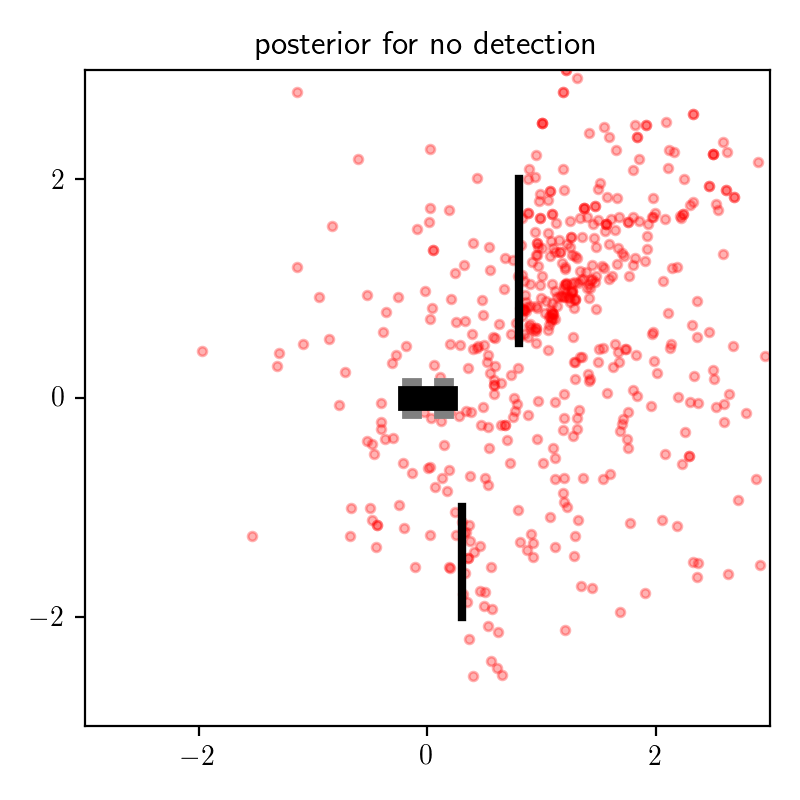
These results make intuitive sense. If there is no detection, then this increases our posterior belief that the object is occluded, which means means the distribution on object location places more mass behind the top occluder. Now consider the posterior results for data sets with is_detection = true and various values for measured_heading:

Recall that our prior belief was that the object was probably in front of the robot (to its right from our top-down perspective). If we receive a detection and a heading measurement in the expected location, then it is probably a true detection. If, on the other hand, we receive a detection and a heading measurement in an unexpected location, then our posterior belief that the detection was a false positive increases, and we consequently place more probability mass on the possibility that the object is indeed behind the occluder. The dynamics of posterior inference are interesting!

Below, I show the results of the symmetrized KL diverence test for the black box variational inference algorithm with variational family q_axis_aligned_gaussian, applied to this model. The teal lines are symmetrized KL divergence estimates for observed data sets where is_detection = true for various values of measured_heading, and the thicker black horizontal line is the symmetrized KL divergence estimate for the observed data set in which is_detection = false.

These results show that the divergence is low when is_detection = false. Also, we see that within observations with is_detection = true, the divergence is generally higher when the measured heading comes from behind the robot. These results make intuitive sense: When is_detection = false, the posterior distribution is unimodal and somewhat similar to the prior, and it is easily captured by an axis-aligned multivariate Gaussian distribution. When is_detection = true and the measured heading comes from behind the robot, the distribution is multimodal because there is significant posterior mass placed on locations behind the top occluder. The variational family we are using cannot approximate this distribution well.

Future work

In addition to the dynamic testing methods like the ones presented here, probabilistic programming systems can also support complementary static analyses. For example, the KL divergences that we estimated above are not guaranteed to be finite, and diagnosing infinite KL diverences using our technique would be difficult. But it is possible to detect this statically in certain cases by analyzing probabilistic programs describing the model and the variational approximation, as shown in a recent POPL paper from Wonyeol Lee, Hongseok Yang and colleagues. Adding libraries to Gen that support a combination of dynamic testing and static analyses of inference code is an ongoing priority for the Gen project.

Another area of future work is in creating domain-specific libraries for testing inference procedures that combine techniques like the one presented here with domain-specific simulators and techniques for generating synthetic data subject to constraints. In particular, integrating ideas from the Scenic system from UC Berkeley with the kind of testing methodology from this post for evaluation of probabilistic perception sytems seems like a fruitfrul direction.

Finally, a characterization of the variance of our symmetrized KL divergence estimator, and applying variance reduction techniques, would be useful.

Related work and references

• Cusumano-Towner, Marco, and Vikash K. Mansinghka. “AIDE: An algorithm for measuring the accuracy of probabilistic inference algorithms.” Advances in Neural Information Processing Systems. 2017. link

• Grosse, Roger B., Siddharth Ancha, and Daniel M. Roy. “Measuring the reliability of MCMC inference with bidirectional Monte Carlo.” Advances in Neural Information Processing Systems. 2016. link

• Grosse, Roger B., Zoubin Ghahramani, and Ryan P. Adams. “Sandwiching the marginal likelihood using bidirectional Monte Carlo.” arXiv preprint arXiv:1511.02543 (2015). link

• Ranganath, R., Gerrish, S. & Blei, D.. (2014). Black Box Variational Inference. Proceedings of the Seventeenth International Conference on Artificial Intelligence and Statistics, in PMLR 33:814-822 link

• Talts, Sean, et al. “Validating Bayesian inference algorithms with simulation-based calibration.” arXiv preprint arXiv:1804.06788 (2018). link

• Geweke, John. “Getting it right: Joint distribution tests of posterior simulators.” Journal of the American Statistical Association 99.467 (2004): 799-804. link

• Neal, Radford M. “Annealed importance sampling.” Statistics and computing 11.2 (2001): 125-139. link

• Lee, Wonyeol, et al. “Towards verified stochastic variational inference for probabilistic programs.” Proceedings of the ACM on Programming Languages 4.POPL (2019): 1-33. link

• Lew, Alexander K., et al. “Trace types and denotational semantics for sound programmable inference in probabilistic languages.” Proceedings of the ACM on Programming Languages 4.POPL (2019): 1-32. link

• Fremont, Daniel, et al. “Scenic: Language-based scene generation.” arXiv preprint arXiv:1809.09310 (2018). link

• Cusumano-Towner, Marco F., and Vikash K. Mansinghka. “Quantifying the probable approximation error of probabilistic inference programs.” arXiv preprint arXiv:1606.00068 (2016). link

• Saad, F.A., Freer, C.E., Ackerman, N.L. & Mansinghka, V.K.. (2019). A Family of Exact Goodness-of-Fit Tests for High-Dimensional Discrete Distributions. Proceedings of Machine Learning Research, in PMLR 89:1640-1649. link